
SoftwareentwicklungUtilities & Energy
Aus einer mobilen LiDAR-Befahrung wird Freileitungsgeometrie
5,6 kmLeiterseil, vektorisiert aus einer Befahrung mit 118,8 Millionen Punkten
Eine Verarbeitungskette, die aus einer rohen Punktwolke aus Mobile Mapping das Freileitungsnetz als zeichenbare Geometrie zurückgibt: Leiterspannfelder, angepasst an die Kurve, der ein hängendes Seil physikalisch folgt, Masten als 3D-Punkte, und jedes Spannfeld mit eigenem Anpassungsfehler, Durchhang und Stützanteil, damit eine prüfende Person die zweifelhaften nach oben sortiert, statt alle anzusehen.
Projektüberblick
Ein Vermessungs- und Geodatendienstleister, der klassifizierte Punktwolken und Geometrie von Netzanlagen an Netzbetreiber liefert. Seine Klassifizierung läuft auf proprietären Desktop-Werkzeugen, je Arbeitsplatz für mehrere Tausend lizenziert, und der Schritt danach, aus klassifizierten Leiterpunkten Liniengeometrie zu machen, mit der CAD- oder GIS-Anwender wirklich arbeiten können, ist noch weitgehend Handarbeit.
- Standort
- Deutschland, remote geliefert
- Dauer
- 4 Monate, von der Bewertung bis zum Produktionslauf
- Zusammenarbeit
- Projektbasiert
- Team
- 1 Ingenieur
Stack
- Data & AI
- PyTorch, Open3D-ML, KPConv, RandLA-Net
- Backend
- Python 3.10+, NumPy, SciPy, scikit-learn
- Survey & CAD
- PDAL, laspy, LAS / LAZ, COPC, GeoJSON, DXF R12, ETRS89 / UTM
- Frontend
- Browser point-cloud viewer with per-span inspection
Die Aufgabe und was sie gelöst hat
Geschäftliche Herausforderung
Die Punktwolkenklassifizierung ist an Desktop-Lizenzen je Arbeitsplatz gebunden, und der Zeichenschritt danach ist Handarbeit. Beide Kosten wachsen mit der Größe der Befahrung statt mit dem Wert des Ergebnisses, was begrenzt, wie viel Arbeit angenommen werden kann.
Was wir gemacht haben
Die Kette läuft auf quelloffenen Komponenten in Python, sodass die Lizenz je Arbeitsplatz den Vektorisierungsschritt verlässt und die Kosten einer größeren Befahrung zu Rechenzeit statt zu Arbeitsplätzen werden. Die Ausgabe erfolgt als GeoJSON und DXF aus derselben Geometrie, sodass sie ohne Zwischenkonvertierung in GIS und CAD landet.
Technische Herausforderung
Ein von einem Straßenfahrzeug aus gescanntes Leiterseil liefert wenige Punkte und kommt in Stücken. Ein einzelnes Seil erscheint als Dutzende durch Verdeckung getrennte Fragmente, parallele Leiter eines Bündels liegen im Grundriss Zentimeter auseinander, und ein Übertragungskorridor darüber ist um eine Größenordnung dünner besetzt als das Verteilnetz auf Straßenniveau, was ihn unter Voreinstellungen für Letzteres vollständig verschwinden lässt.
Was wir gemacht haben
Klassifizierte Leiterpunkte werden zu Kandidaten für Spannfelder gruppiert, parallele Leiter in einem gemeinsamen Korridor werden über ihren seitlichen Versatz und den Durchhang im Querschnitt getrennt, statt als eine dicke Linie angepasst zu werden, und jedes Spannfeld erhält die Kettenlinie, der ein hängendes Seil tatsächlich folgt, mit Parabel und Geradenstücken als Rückfallebene. Masten laufen einen eigenen Weg und werden nur im Grundriss gruppiert, damit ein vollständiges vertikales Bauwerk ein einziges Objekt bleibt. Durch Verdeckung zerbrochene Spannfelder werden wieder zusammengeführt, wo die Stücke auf einer Linie liegen und die erneute Anpassung trägt.
Herausforderung in der Umsetzung
Niemand prüft bei einer Befahrung dieser Größe jedes Spannfeld in 3D. Eine Ausgabe, die nicht sagen kann, welchen ihrer eigenen Spannfelder zu misstrauen ist, muss vollständig geprüft werden, und damit ist der Handaufwand wieder da.
Was wir gemacht haben
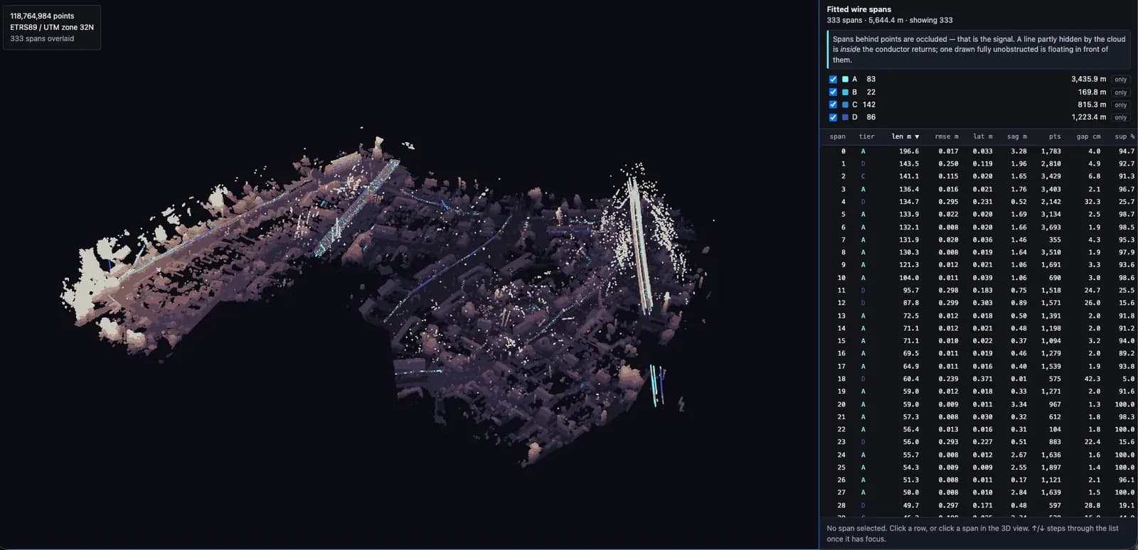
Jedes Spannfeld trägt eigene Qualitätskennwerte, Anpassungsfehler auf beiden Achsen, Durchhang, Punktzahl, Lückenprofil und den Anteil seiner Länge, der tatsächlich durch Messpunkte gestützt ist, und der Prüf-Viewer sortiert und filtert nach jedem davon. Die Prüfung beginnt bei den Spannfeldern, die Zweifel verdienen, statt bei Spannfeld null.
Spans behind points are occluded, and that is the signal. A line partly hidden by the cloud is inside the conductor returns; one drawn fully unobstructed is floating in front of them.
Warum wir
Die Messungen verschoben immer wieder den Engpass, und wir veröffentlichten jeweils, wohin er sich verschoben hatte, statt der Zahl, die der gerade bearbeiteten Stufe schmeichelte. Die Geometrie war nie die Grenze, sondern die Trefferquote der Klassifizierung. Und zwei Voreinstellungen, eine Höhenobergrenze und ein Verbindungsabstand, verwarfen einen ganzen Übertragungskorridor, bevor irgendetwas Nachgelagertes ihn sehen konnte. Das findet nur, wer die Verarbeitungskette so instrumentiert, dass man mit ihr streiten kann.
- Phase 1
Bewertung der Architekturen
Zwei Deep-Learning-Architekturen zur Segmentierung wurden an gängigen Punktwolkendatensätzen aus Luft- und Fahrzeugbefahrung verglichen, mit selbst gemessenen Kennwerten je Klasse statt Zahlen aus Veröffentlichungen, um die Grundlage für ein produktives Werkzeug zu wählen.
- Phase 2
Vektorisierungskette
Gruppierung der Spannfelder, Trennung der Bündel, Anpassung der Kettenlinie und der eigene Weg für Masten, mit Export nach GeoJSON und DXF, geprüft gegen Referenzdaten auf einer öffentlichen Vergleichskachel.
- Phase 3
Trefferquote und Kachelmaßstab
Schwellenwerte auf den Wahrscheinlichkeiten sowie ein vom Klassifikator unabhängiger Schritt zur Korridorwiederherstellung, der über Geometrie statt über Bewertungen ergänzt, dazu gekachelte Inferenz, damit eine ganze Kachel statt eines Ausschnitts verarbeitet werden kann.
- Phase 4
Produktive Befahrung
Die Kette lief von Anfang bis Ende auf einer Mobile-Mapping-Befahrung mit 118,8 Millionen Punkten, mit an diesen Daten neu hergeleiteten Voreinstellungen und einer 3D-Prüfung des Ergebnisses.
Ergebnisse
Zwei Voreinstellungen entschieden darüber, ob der Übertragungskorridor der Befahrung im Ergebnis existierte oder gar nicht: eine Höhenobergrenze, die rund eine Viertelmillion Punkte oberhalb von zwanzig Metern verwarf, bevor die Anpassung überhaupt lief, und ein Verbindungsabstand, kürzer als die Lücken, die Verdeckung in einem von der Straße aus gescannten Seil hinterlässt. Beide anzuheben brachte einen halben Kilometer hochvertrauenswürdiger Linien zurück, den kein früherer Export enthielt.
5.644 mLeiterseil vektorisiert
333Spannfelder angepasst und nach Vertrauen bewertet
2,2 cmmittlerer Abstand von einem angepassten Spannfeld zum nächsten Messpunkt
118,8 Mio.Punkte in einer einzigen Befahrung verarbeitet
| Kennzahl | Vorher | Nachher |
|---|---|---|
| Leiterseil vektorisiert | 4.748 m | 5.644 m |
| Spannfelder angepasst und nach Vertrauen bewertet | 317 | 333 |
Total length is the obvious aggregate and it prefers the wrong answer. Only the corridor-specific figure exposes conductors chaining across each other instead of along themselves.
Was wir geliefert haben
Anpassung der Kettenlinie je Spannfeld
Jeder Leiter erhält die Kurve, der ein hängendes Seil physikalisch folgt, mit Parabel und Geradenstücken als Rückfallebene, und meldet seinen eigenen Restfehler.
Trennung von Leiterbündeln
Parallele Leiter in einem gemeinsamen Korridor werden über seitlichen Versatz und Durchhang im Querschnitt getrennt, statt als eine dicke Linie durch die Mitte angepasst zu werden.
Zusammenführen bei Verdeckung
Ein in Fragmenten ankommendes Seil wird wieder zusammengefügt, wo die Stücke auf einer Linie liegen und die erneute Anpassung trägt, statt als Bruchstück-Haufen zum Nachzeichnen geliefert zu werden.
Vertrauensstufen je Spannfeld
Jedes Spannfeld wird bewertet und trägt Punktzahl, Stützanteil, Lückenprofil, Durchhang und beide Fehlerachsen, sodass eine Prüfung dort beginnen kann, wo Zweifel angebracht sind.
Mastextraktion
Masten werden nur im Grundriss gruppiert, sodass ein vollständiges vertikales Bauwerk ein Objekt bleibt und nicht nach Höhe zerfällt, und werden als 3D-Punkte mit ihrer Höhe exportiert.
Ausgabe für CAD und GIS
GeoJSON-Linienzüge und DXF-Polylinien aus derselben Geometrie erzeugt, dazu ein Browser-Viewer, der die Spannfelder durch die Punktwolke zeichnet, an die sie angepasst wurden.
Im Detail
Ein Mobile-Mapping-Fahrzeug befährt ein Netz und liefert hundert Millionen Punkte zurück. Irgendwo in dieser Wolke steckt das Freileitungsnetz, und was der Kunde tatsächlich braucht, sind nicht die Punkte, sondern die Linien: jedes Leiterspannfeld als zeichenbare Kurve, jeder Mast als Punkt, in einer Datei, die sich in CAD und in GIS öffnen lässt.
Dorthin zu kommen ist eher ein Geometrie- als ein Machine-Learning-Problem. Klassifizierte Leiterpunkte werden zu Kandidaten für Spannfelder gruppiert; parallele Leiter in einem gemeinsamen Korridor, die im Grundriss nur Zentimeter auseinanderliegen, werden anhand ihres seitlichen Versatzes und der Form ihres Durchhangs im Querschnitt getrennt. Jedes so entstandene Spannfeld erhält eine Kettenlinie, also die Kurve, die ein unter seinem eigenen Gewicht hängendes Seil physikalisch einnimmt, mit einfacheren Rückfallebenen, wo die Daten sie nicht tragen. Masten laufen einen parallelen Weg und werden nur im Grundriss gruppiert, damit ein vollständiges vertikales Bauwerk ein Objekt bleibt und nicht nach Höhe in Scheiben zerfällt.
Von einem Straßenfahrzeug aus gescannt, liefert ein Seil in fünfundzwanzig Metern Höhe nur wenige Punkte und kommt als Bruchstück-Haufen an: Dutzende Fragmente, überall dort getrennt, wo etwas zwischen Sensor und Seil stand. Diese Stücke werden wieder zusammengeführt, wo sie auf einer Linie liegen und die erneute Anpassung trägt, und genau das macht aus einer Streuung von Stummeln wieder ein Spannfeld.
Zwei Voreinstellungen dieser Befahrung waren mehr wert als jede Änderung am Algorithmus. Eine auf das Verteilnetz auf Straßenniveau abgestimmte Höhenobergrenze verwarf jeden Punkt oberhalb von zwanzig Metern, bevor die Anpassung lief, und der Übertragungskorridor liegt bei zweiundzwanzig bis dreißig. Und der beim Zusammenfügen zerbrochener Stücke erlaubte Abstand war kürzer als die Lücken, die Verdeckung in dieser Höhe tatsächlich hinterlässt, sodass selbst ein sauberes Zusammenfügen strukturell unmöglich war. Beides anzuheben brachte die Befahrung von 4.748 auf 5.644 Meter Leiterseil und lieferte elf hochvertrauenswürdige Spannfelder vollständig oberhalb von zwanzig Metern, wo frühere Exporte gar keine hatten.
Nichts davon nützt ohne eine Möglichkeit, ihm zu misstrauen. Jedes Spannfeld wird mit eigenen Zahlen geliefert, Anpassungsfehler auf beiden Achsen, Durchhang, Punktzahl, Lückenprofil entlang seines Verlaufs und der Anteil seiner Länge, der wirklich durch Messpunkte gestützt ist, und der Prüf-Viewer sortiert nach jedem davon. Die Verdeckung wird so zur Prüfgröße statt zum Ärgernis: Ein hinter den Punkten gezeichnetes Spannfeld liegt innerhalb der Leiterpunkte, eines, das frei davor schwebt, nicht.
Zahlen Sie je Arbeitsplatz, um Linien durch eine Punktwolke zu zeichnen?
Klassifizierung und Vektorisierung sind trennbare Probleme, und das zweite ist überwiegend Geometrie. Buchen Sie ein technisches Gespräch, und wir sehen uns eine Kachel Ihrer Daten an und sagen Ihnen, welche Hälfte sich zuerst zu automatisieren lohnt.